| |
EXERCISES ON TEST GENERATION AND FAULT DIAGNOSTICS
Objectives
The main aim is to provide the basic ideas about testing and diagnosis of digital circuits. In particular, the work focuses on the following issues: 1) what testing is and how it can be done 2) how diagnosis can be performed and 3) what is the difference between testing and diagnostics.
Introduction
Testing a circuit means evaluating whether it works correctly. This is normally done by applying input test vectors, and observing the produced output value. If a fault is found, it is considered as an incorrect behavior of the circuit (with respect to that which has been assumed as the correct). To perform testing and thereupon to do the diagnosis we need to choose the fault model, which we will use in the future. The most popular model is called the stuck-at fault model. We are going to use it during our laboratory work. When a line is stuck-at a given value (0 or 1) then it is said that the stuck-at model to be used here.
A common
measure to evaluate the effectiveness of a given test set is the fault coverage,
which is the percentage of faults, which are detected by the set against
the full set of faults. Of course, the fault coverage of 100% is always
desirable but rarely attainable in most practical circuits.
Quite frequently we could face with the problem of generating a test vector for a fault. The problem complexity grows exponentially with the size of the circuit. The software tools addressing this problem are known as ATPGs (Automatic Test Pattern Generators). Some popular automatic tools that are used for test generation are deterministic test pattern generator, random test pattern generator and others.
Test generation and fault diagnosis are strongly connected with each other. We could not diagnose without testing. Consider the manufacture process of 999 items of the same circuit. After a circuit has been manufactured, it must be tested. As a result of a testing procedure, let's say for instance, we have got 333 faulty circuits with the same fault occurred. The manufacture process itself must be the reason for this fault appearance (for example, such fault as the bridging fault is said to be occurred when two or more wires that are normally independent become electrically connected). Thereupon the diagnosis aims at locating the cause of the fault. After the diagnosis, some necessary improvements have to be done in the manufacture process.
Work description
The training will be done using the Gate Level Test and Diagnosis Applet. You will need to choose a circuit you are going to practice with (the variant of this circuit corresponds to the last number of your matriculation). All circuits are 100% testable, they all have 5 inputs and 2 outputs and the number of gates can vary from 8 to 10. To do training you will need to execute following operations (see Steps). In this laboratory work we are not going to study any ATPGs, instead, we will practice with pseudorandom test generation using LFSR (Linear Feedback Shift Register) and manual (deterministic) test generation. The last step you must do in the work is the fault diagnosis using different approaches, like guided probe testing and combinational fault diagnosis that is based on fault table analysis. In the diagnosis part you must try to figure out by your own the rules and methods to be used in order to accomplish required tasks. Also, there will be given an Example, where you can see all the steps performed.
1. Pseudorandom test pattern generation using LFSR.
1.1 Run the gate level test applet and then under Circuit selection menu choose your variant of the circuit. Afterwards on Control Panel choose LFSR and then BILBO (Built-In Logic Block Observer) mode. Select the LFSR length (bits); let it be the same as the number of inputs of your circuit. Next randomly choose the configuration for LFSR: enter initial state values and feedback configuration.
1.2 Insert the number of test vectors you need to generate; let's choose the step of 5 test vectors. Then push the button Run LFSR. Afterwards under Working modes menu choose Fault simulator to fill the fault table. For the next, see the applied coverage, if it is not 100%, repeat the step 1.2 again with increased number of test vectors with a step 5 until you have reached the desirable 100% of fault coverage. If it does not help (you have not still reached 100% of fault coverage), try to choose another configuration for LFSR and then repeat the step 1.2 again. At last, if you have reached 100% of coverage, please write down the final configuration for LFSR and go directly to the step 2.
1.3 If you were unlucky and after several changes in the configuration of LFSR 100% of fault coverage was not still achieved, use the primitive polynomial. The length of the LFSR sequence is determined by its characteristic polynomial. An N-degree polynomial yields a maximal length cycle
if it is a primitive polynomial (31 vectors for 5-bit input). Only a primitive polynomial guarantees a maximal-length sequence. For the 5-input circuit, the primitive polynomial has the second and the fifth bits used for feedback. Repeat the step 1.2 again.
2. Fault table study.
2.1 Find 5 or more easily tested faults, and then all hard-to-test faults. Note that there are some faults in the circuit that can be tested only by unique test vectors. These faults we will consider as the hard-to-test faults.
2.2 Write down the test vectors that discover the hard-to-test faults.
2.3 If it is possible, try to find the redundant test vectors and then delete them. We will consider a redundant test vector as a vector that does not increase the fault coverage. In the same way, a test vector may be redundant if other test patterns in the fault table cover all the faults that were tested by this vector. By deleting some redundant vectors, we will decrease the cost of our test.
3. Manual (deterministic) test pattern generation.
3.1 On Control Panel choose Manual. Afterwards, you can act in two different ways: by applying a test pattern directly from Control Panel or by choosing Generate testvectors under Working modes menu in order to detect the specific fault you want to insert into the circuit. If you have chosen the second method, then you need to propagate this fault to the output and observe the produced output value. This can be done by clicking on the values of checkpoints and detecting the value you need to choose. In order to propagate the fault to the output, you need to make those gates transparent through which the fault is passing. While propagating the specific fault, try to test as much faults as you can by applying the same test vector. Continue generating test vectors until you have reached the desirable 100% of fault coverage.
3.2 After you have inserted test vectors that give you 100% of fault coverage, check the possibility of deleting some of them. Probably, you can do it without losing the fault coverage. Try to construct as short complete (100% of fault coverage) test as you can. Afterwards, evaluate the cost (the quality) of your test.
4. Guided probing diagnosis.
4.1 After the simulation of test vectors from the previous step 3, choose Guided probing under Working modes menu to enter this mode. Now you can randomly insert the fault into the circuit.
4.2 Select a vector marked as 'N' and click on testpoints for measuring signal values. Remember, the principle of guided-probe testing is to backtrace an error from the primary output where it has been observed to its source.
4.3 As the most time-consuming part of guided-probe testing is moving the probe, you should try to reduce the number of probed lines. Try to make as less number of clicks as you can.
4.4 Formulate some rules or methods to minimize the number of probes (not mentioned in an Example).
4.5 Construct a diagnostic tree for the specific vector (review the theory).
5. Combinational fault diagnosis (fault table based).
5.1 Choose Combinational fault detection under Working modes menu. Again, like it was done in the previous step 4, you should randomly insert the fault into the circuit.
5.2 By clicking on vectors, select (use Ctrl button pressed to pick two or more test vectors) as less number of test vectors as you think it will be enough in order to find the fault location.
5.3 Try to formulate some rules for the selection of test vectors (not mentioned in an Example).
5.4 If you cannot localize the fault even after all the vectors have been selected, construct one or more additional diagnostic test vectors (review the theory).
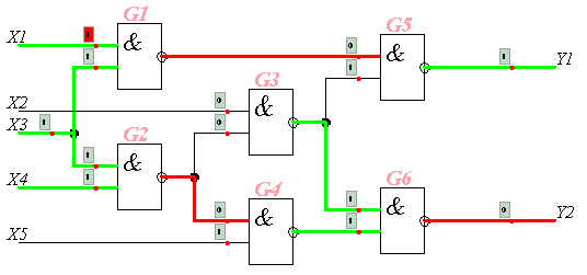
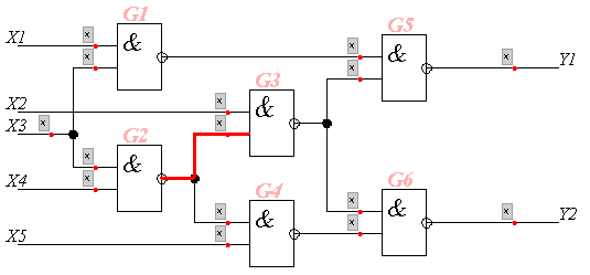
Here we will follow the Steps and show how one can follow them. In this example we will use a small 5-input and 2-output circuit that has 6 gates in it (ISCAS c17 under Circuit selection menu).

Steps
1. Pseudorandom test pattern generation using LFSR.
1.1 When all selections are done, we set to the step 1.2.
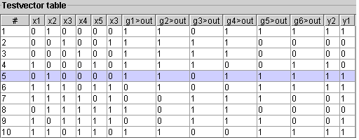
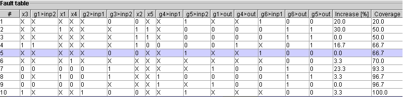
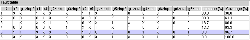
1.2 First 5 vectors generated by LFSR have given the fault coverage of 66.7%; it is not bad since we have covered more than a half of all possible faults only by 5 test vectors. But our goal is 100% and therefore let us add 5 test vectors more (since we have chosen the step of 5 test vectors). After the simulation of 10 test vectors, we are lucky to have the desirable 100% of fault coverage. Now, we can go straight to the step 2. The test vector table and the produced fault table are illustrated below.
2. Fault table study.
2.1 Now we find some easily tested faults, and then hard-to-test faults. For the first, we can outline, for instance: g5>out (sa-0), g6>out (sa-0 and sa-1), g6>inp1 (sa-0), g4>out (sa-0). We consider an easy tested fault as a fault that can be tested by maximum number of test patterns in comparison with the number of vectors, which can cover other faults. Thus, g5>out (sa-0) is tested by 6 test vectors. As there are no other faults that can be tested by 6 test patterns, we have chosen the faults that are testable by 5 patterns. Therefore, g6>out (sa-0 and sa-1), g6>inp1 (sa-0), and g4>out (sa-0) are tested by 5 test vectors. For the hard-to-test faults, we can choose, for instance: x4 (sa-1), g2>inp1 (sa-1). Only unique test vectors detect these two faults. There are more hard-to-test faults, which we do not show here, but in your variant of circuit you should find them all.
2.2 Here we write down the test vectors that discover the hard-to-test faults: for the fault x4 (sa-1) - 11101, for the fault g2>inp1 (sa-1) - 11011. We took them from the testvectors panel.
2.3 It is clear that the third, the fifth and the ninth test patterns do not increase the fault coverage (see increase [%] column in the fault table), therefore we can easy delete them. The rest test vectors we have to leave, since they test some unique faults.
3. Manual (deterministic) test pattern generation.
3.1 Suppose, we have chosen Generate testvectors under Working modes menu. Let's choose the fault x1 (sa-0) and insert it into the circuit. Now we need to propagate this fault to the output Y1. Thus, g1>inp2 must have '1' value and g5>inp2 must be '1' valued too. By applying these values, we make transparent g1 and g5 gates through which the fault x1 (sa-0) is propagating. We must also try to cover as much faults as we can. For example, if we drive the input x5 to a '0' value, we could not test x4, g2>inp1, and g4>inp1, because by applying this value, we make the NAND gate not transparent, so that these faults could not influence its gate output.
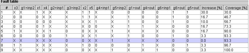
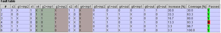
3.2 Suppose, we have got 100% of fault coverage. Now we should check the possibility of deleting redundant vectors. Let's take a look at the fault table. We can see that the seventh test vector has not increased the fault coverage therefore we can delete it. Also, we can delete the second and the third test vectors, because other test vectors in the fault table could test the same faults that these two patterns can test. Thus, we have decreased the cost of our test from 9 to 6 test vectors (see the second figure below).
4. Guided probing diagnosis.
4.1 Let's randomly insert the fault into the circuit.
4.2 Then we select at least one of the vectors marked as 'N' (not passed, which means that the fault has been detected at the output(s)).
4.3 Now we must move the probe in order to backtrace an error from the primary output to its source. In the same way we are trying to make as less number of probes as we can. Let's try one of the outputs, Y2. We were lucky to guess and the fault is observable at this output (red line of Y2 is indicating this). Next we must check one of the inputs of gate g6. Okey, let us try the second input, g4>out. This input is red too. The next step is to move further and check one of the inputs of gate g4. In this case, we can say for sure that x5 is not faulty, because g4>inp1 that is '0' valued, which makes the other NAND input x5 unobservable. Hence, only input g4>inp1 can influence the gate's output. Therefore, we select it and find that it is faulty. Now it is time to probe one of the inputs of gate g2. Let it be the first input, g2>inp1. The grey line is indicating that there is no error on it. Okey, but we still must check the second input of gate g2. The randomly inserted error could be there. After clicking on the second input of gate g2, we find that it is grey colored too. We have realized that our supposition was wrong. Now we can say for sure that the source of the fault is g4>inp1. We have needed only 5 probes to localize this fault. From this moment, we can stop our diagnostic process, since we have backtraced the fault from the primary output Y2 where it has been observed to its source, g4>inp1.

5. Combinational fault diagnosis (fault table based).
5.1 Let us randomly insert the fault into the circuit.
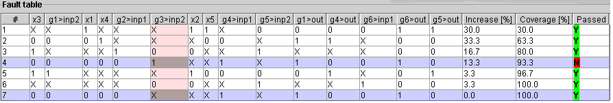
5.2 Now by clicking on vectors, we must select as less number of test vectors as it will be enough in order to localize the randomly inserted fault. For this, see the figures below: the fault table and the circuit, where the fault is graphically illustrated. In this case, by selecting all 6 vectors we cannot localize the randomly inserted fault (the diagnostic resolution is too low, and it is 4 faults at the moment). The fault table shows that there are still 4 faults, x4 (sa-0), g2>inp1 (sa-0), g3>inp2 (sa-1) and g4>inp1 (sa-1). Only one of them is a real fault. For this case, we must add such a pattern that detects some of these 4 suspected faults, but at the same time does not detect others.

5.2 (continue) In this way, by applying an additional diagnostic test vector, we can decrease the list of the suspected faults. After that, let's hope that we will find our randomly inserted fault. Thus, let us add an additional test vector 10111. This test pattern tests 3 suspected faults: x4 (sa-0), g2>inp1 (sa-0), and g4>inp1 (sa-1). As a result, in the new fault table we can see that the last vector that was added is marked as 'Y' (passed, which means that the fault has not been detected at the output(s)), therefore these 3 mentioned faults are out of the suspicion now. Thus, it is easy to assume that the randomly inserted fault has occurred on g3>inp2 and it is stuck-at 1. For this, see the figures below: the new fault table with added seventh test vector and the circuit, where the randomly inserted fault is graphically represented.
| |
|
|
Last update: 28 July, 2004