1. Test Generation       1.1. Example 2. Design Error Diagnosis 3. Built-in Self-Test 4. Design for Testability

 

1. TEST GENERATION

Objectives
To practice with manual and automatic test pattern generation. To perform fault simulation and to analyze the simulation information. To compare the efficiency of different methods and approaches.
 

Introduction
After a circuit is manufactured it has to be tested for manufacturing defects (physical faults) to ensure it has been fabricated correctly. There is a number of various methods used in test generation (TG). For example, deterministic methods, random and pseudorandom TG, genetic algorithms (and other non deterministic search) based TG, combined TG, etc. Each technique has its advantages and drawbacks. The efficiency of TG method can be significantly improved for a some classes of circuits if we can force it using the information about the functionality or the structure of the circuit. This is the clue why manual TG sometimes can give better results than automatic methods. For example, any ripple-carry adder, no matter how wide it is, can be tested with 8 test vectors only. A human can easily compose such a test. However, automatic test pattern genrators (ATPG) can hardly provide a test of such a small length. The main drawback of manual test generation, however, is the dramatically low speed of the process.

Work description
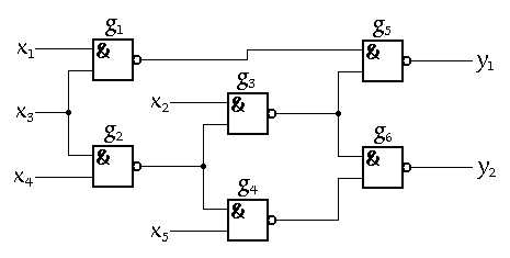
In this work we are going to study and compare different TG methods. There are three circuits to be tested. The first one is a relatively small random circuit with 5 inputs and 2 outputs. The second is a full 8-bit ripple-carry adder with 17 inputs (two 8-bit operands and the carry in) and 9 outputs (one 8-bit result and the carry out). The third circuit is to be chosen from the list of comparatively complex ISCAS '85 benchmarks.

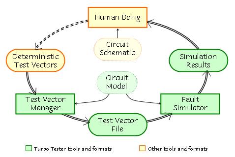
First of all, a manual test pattern generation (random and deterministic) is to be practiced with. The following diagram shows in general what has to be done at this step. We took the deterministic test generation as the example here.

You begin with the selection of the circuit under test and calculate the first test vector (or several vectors at once). For that you have to use one of the methods you have been taught during the lectures. Otherwise, you can use the method from the theoretical notes. This vector must be then converted into a special format and saved in the test vector file. All these technical things are performed by the vecmanager tool. After fault simulation you will receive information about signals in the circuit and faults on these signals that are covered by your test. If the required test coverage level has not been reached yet, the whole process must be repeated.

There are also some automatic tools (ATPGs) to be used for test generation in this work:

• Deterministic test pattern generator
• Genetic algorithm based test pattern generator
• Random test pattern generator

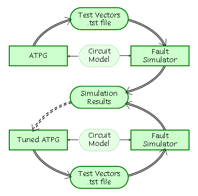
A similar diagram (below) illustrates the workflow. The process starts after the circuit and the corresponding ATPG has been chosen. First, the ATPG has to be run with default settings. Then test vectors are fault simulated and the results are registered and saved. The next phase is started with the adjustment of the ATPG. Everything is repeated then with the new ATPG settings. The ATPG can be tuned further and process is repeated again for several times until the target test quality (test length/cover) is achieved.

In the case of the deterministic ATPG, there is no possibility of tuning in order to achieve a shorter test with the same fault coverage. Only the coverage can be improved (if possible) by further adjustment. For some circuits the maximum coverage is always achieved with default options and no tuning needed at all. In that case we can use the test compaction technique. It uses the fault table to select the minimal number of test vectors sufficient to cover all the faults. Remaining vectors can be removed without the fault coverage reduction.

The tasks for Test Generation laboratory work are summarized in the following table, where the sign denotes the task to perform.

TABLE 1

	small	adder	ISCAS'85
Random manual			—
Algoritmic manual			—
ATPG	—

After the mentioned tests are obtained the cost of test generation can be calculated. There are different methods used for that. We will use the following equation:

Cost = C_v + C_t + C_%

a, b, and c are to be chosen by the following rules:
– 10 additional test vectors can be justified by 1% of fault coverage gain;
– we agree to spend 10 seconds more to generate 1-vector shorter test.
 

Steps

1. Apply manually as many randomly chosen test patterns as you think it will be enough for the first circuit. However, remember that the goal is to acquire a test with possibly better fault coverage using possibly smaller amount of test patterns. You can try sevral combinations and numbers of patterns.
2. Use some heuristics or certain algorithms to make an even better test (if it is possible) than you have already acquired. Refer to the theory for the test generation methods.
3. Repeat the steps above (1, 2) for the adder. Note, that it is too large to use the gate level manual test generation methods during the step 2. Use functional level methods instead.
4. Use the three listed above automatic test generation tools and acquire three tests more. Run the ATPGs with default options.
5. Run the "genetic" and "random" ATPGs in a tuned mode. Try different settings to achieve shorter test, than you received at the previous step. Run the deterministic ATPG without tuning again and perform the test compaction using the optimize tool.
6. Compare the length and fault coverage for all the tests and decide which test and test generation method (or a number of tests and methods) is the best for the given circuit. Why?
7. Repeat steps 4,5,6 for one of the ISCAS '85 benchmarks.
8. For the last circuit, calculate the cost of testing for each of the used method.

Here (as well as in all examples of this course) we will follow the Steps and show how one can follow them. The circuit to be used in this example is a small ISCAS '85 benchmark c17 (c17.agm).

1. First of all let's try random patterns and see how good is the fault coverage they can provide. In Table 2, some random vectors are given. Using vecmanager tool we can apply them to the circuit and perfom fault simulation.

TABLE 2

	x1	x2	x3	x4	x5
Pattern 1	1	0	1	0	1
Pattern 2	0	1	0	1	0
Pattern 3	0	0	0	0	0
Pattern 4	1	1	1	1	1

The obtained cover is 90.91 % (20 out of 22). Not bad but these four vectors are not enough for the given circuit since our goal is 100% fault coverage (if possible) and therefore let us add one pattern more (use vecmanager again). Let it be the pattern 00111. After that the fault simulator reports higher coverage of 95.45 % (21/22). Still not enough. Okay, let's add then, for instance, the pattern 11100. Again 95.45 % (21/22), which means that this pattern doesn't improve the coverage and, therefore, we are going to remove it and select another one. Let it be 10011. This time the simulator reports 100% (22/22). The final result is reflected in the following table.

TABLE 3

	x1	x2	x3	x4	x5
Pattern 1	1	0	1	0	1
Pattern 2	0	1	0	1	0
Pattern 3	0	0	0	0	0
Pattern 4	1	1	1	1	1
Pattern 5	0	0	1	1	1
Pattern 6	1	0	0	1	1

We have a pure random set of 6 vectors, giving the 100% fault coverage. However, it is maybe possible to compose a shorter test. Let's try other techniques and see if they can improve the test.

2. Composition of the shortest possible test by hand is a difficult task. However, some heuristics on that topic exist. Here we will try to achieve the goal by composing each vector so that it will cover as much faults in the circuit as possible. Refer to the theory for more details on that topic. Here (Table 4) is an example of a test with 100% coverage consisting of 4 vectors only. It is shorter (better) than the random test above by 1/3 of the length.

3. The procedure for the adder is quite similar to the work described above except the step 2. At this step try functional test generation methods. There is, for instance, a method which gives 100% fault coverage for the ripple-carry adder with only 8 vectors.
   
   
4. Now let's examine the automatic test pattern generators (ATPG) and see how good are the tests they can provide. Consider again the c17 circuit. First we are going to run ATPGs with their default options (usually the fastest) and then try to adjust them to get shorter tests (step 5).

   In Table 5, the experimental results for three ATPG types are given. The first row indicates used options (default and tuned). The three lowest rows reflect the information concerning the number of vectors and the generation time for the three ATPGs.

The deterministic ATPG with default options gives a six-pattern test which is longer than that we composed manually. However, we can use the test compaction in order to reduce the number of vectors, at the same time keeping the fault coverage level unchanged. For that we have to run ATPG once again with option -fault_table (generate -fault_table c17). This option allows the fault table used for the test compaction to be saved together with test vectors into the c17.tst file. Then we run optimize c17 command. The results are given in Table 5. As you can see, there is no test reduction this time. However, for larger circuits you should observe it.

The next ATPG is the genetic algorithm-based one. It gives sometimes five, sometimes four vectors with default options. To achieve a shorter test we can set bigger population size. For example the setting -popul_size 64 (instead of -popul_size 32 by default) gives usually a four-vector test. At the same time the generation time grows almost twice. That is, we receive a better test on the cost of the time used for the test generation. What is really better (shorter test or shorter time) in this situation? The question can be answered after the calculation of the test generation cost (step 8).

The random ATPG gives the worst test (6 patterns) when run with default options. However, adjusted (random -pack_size 2 -select_max 1 c17) it is also able to generate the test with minimal length (4 patterns). The generation time in the latter case has also increased.

6. So far we have composed two tests manually (random and deterministic) and three tests using automatic tools. At this step our task is to compare the quality of studied methods, which includes the test length, fault coverage and test generation speed. For this small circuit all the methods were relatively equal. What results did you in your work? For better reasoning the cost calculation is needed (step 8).
    
7. ISCAS benchmarks are quite large to start composing a test for them manually. Therefore, follow the steps 4,5, and 6 only.
    
8. Here is an example of cost calculation for genetic algorithm. Let's take here a = b = c = 1 (note, that in your case they will be different!). For test generation with default settings the cost will be the following: Cost_def = C_v + C_t + C_% = 5 + 0.09 + 0 = 5.09. Test generation cost for the adjusted genetic ATPG is Cost_adj = 4+ 0.17 + 0 = 4.17. This means that for the selected parameters a, b, and c the second method will be better.

Last update: 27 July, 2004